Modeling with Gaussian Processes: Enhancing Physical Models with Embedded Machine Learning
In many scientific and engineering domains, physical models—based on first-principles or mechanistic assumptions—
often leave out complex, unknown, or poorly understood phenomena. Harappa Modeling introduces a hybrid strategy that
augments these models using Gaussian Processes (GPs) to capture and correct the residuals left by incomplete physics.
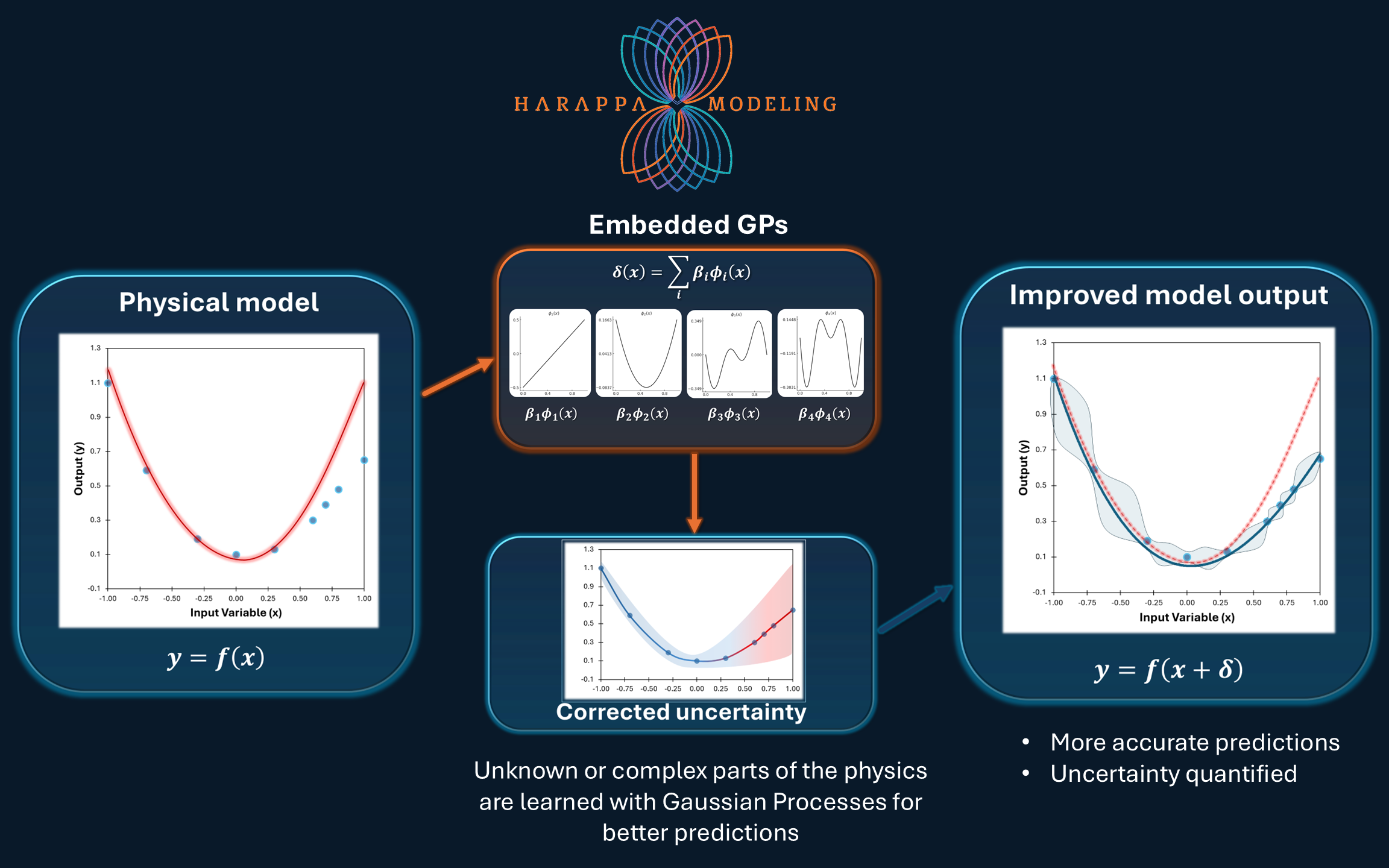
1. Physical Model
We begin with a physical model:
y = f(x)
This model provides a baseline prediction, but due to simplifications or missing physics, a discrepancy
exists between model predictions and observed data. This discrepancy represents what the physics-based model fails to
capture.
2. Discrepancy
To make up for missing physics we incorporate a data-driven function:
y = f(x, δ)
This hybrid model will yield more accurate predictions if we can learn the unknown function δ(x).
3. Residual Minimization with GPs
We model the function δ(x) using a set of basis functions:
δ(x) = ∑ β_i φ_i(x)
Here, each φ_i(x) is a basis function derived from a Karhunen–Loève decomposition of a GP kernel, and the coefficients β_i are
stochastic coefficients learned using Markov sampling. This approach provides a data-driven, flexible correction to the physical model while
preserving interpretability. The GP may represent a well-defined physical quantity such as a diffusivity or rate constant.
4. Quantified Uncertainty
By integrating the GP-based correction, we not only improve the mean prediction but also estimate uncertainty bounds
around the output. This is especially important for dynamic problems.
Why Use GP-Based Residual Correction?
• Bridges the gap between theory and data
• Captures unmodeled dynamics using a non-parametric Bayesian framework
• Improves predictive performance while respecting physical constraints
• Delivers credible intervals and interpretable corrections
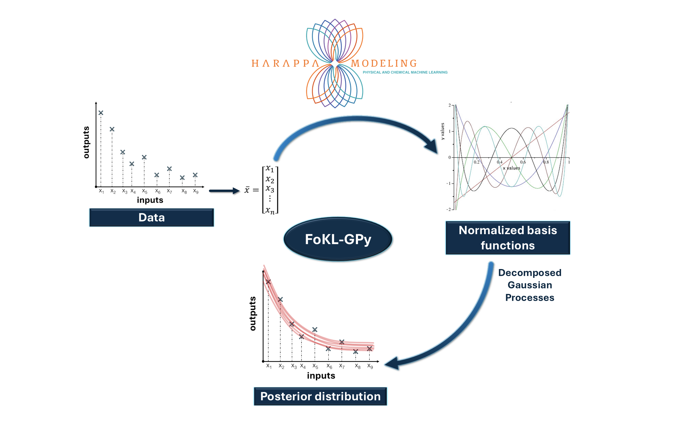
FoKL-GPy: Forward Variable Selection with Karhunen–Loève Decomposed Gaussian Processes in Python
This diagram illustrates the workflow of the FoKL-GPy framework — a novel approach that leverages Karhunen–Loève (KL)
decomposition of Gaussian Processes for efficient, interpretable modeling.
Gaussian processes are powerful kernel-driven nonparametric interpolation engines, which make them ideal for learning the underlying structure of continuous datasets with relatively low input dimensionality. However they are typically slow to train and difficult to evaluate within the context of other models. The Karhunen-Loève theorem enables a decomposition of the kernel into a set of deterministic basis functions, greatly accelerating both training and evaluation. A novel forward varlable selection method keeps the expansion tractable.
the article
the repo
Case Studies
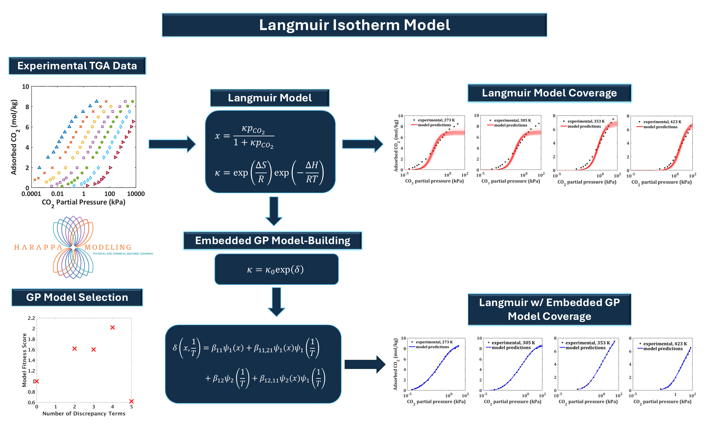
Thermodynamic Data-Driven Framework for CO_2 Adsorption
This schematic illustrates a modeling approach that augments the classical Langmuir isotherm with Gaussian Process (GP)
regression to improve accuracy and capture temperature- and pressure-dependent discrepancies in gas adsorption data.
Experimental TGA Data
Thermogravimetric analysis (TGA) experiments measure CO_2 uptake as a function of partial pressure and temperature. The multicolor dataset on the left displays adsorption curves over a range of pressures and temperatures.
Langmuir Model
The Langmuir isotherm describes adsorption onto a homogeneous surface. The core equation relates adsorbed amount x to pressure pCO_2, with an equilibrium constant κ that depends on temperature via van’t Hoff's relation involving enthalpy
(∆H) and entropy (∆S) terms.
Langmuir Model Coverage
Initial predictions using the pure Langmuir model (top right) show reasonable but imperfect agreement with experimental
data, highlighting model-form discrepancies especially at lower temperatures and higher pressures.
Embedded GP Model-Building
To address these discrepancies, the model embeds a GP correction δ(x, 1⁄T) into the expression for κ, treating it as a
temperature- and coverage-dependent perturbation:
κ = κ_0 exp(δ)
GP basis terms (bottom center) are chosen via model selection (bottom left), using a fitness score to balance complexity
and accuracy.
Langmuir with Embedded GP Coverage
The improved hybrid model (bottom right) yields accurate predictions across all temperatures, better aligning with
experimental observations and offering improved extrapolation confidence.
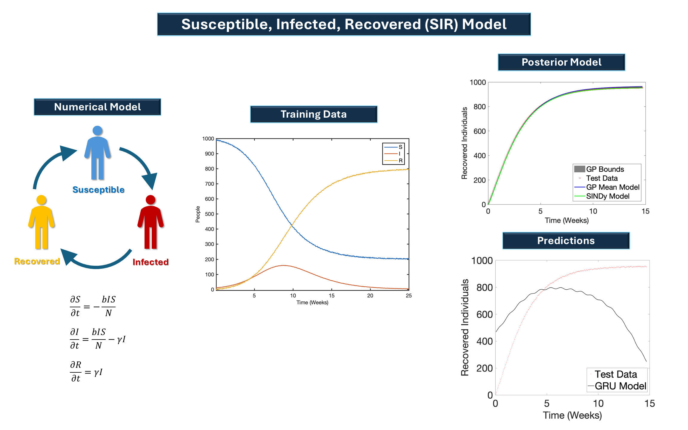
Susceptible-Infected-Recovered (SIR) Model: Data-Driven Epidemiological Forecasting
This figure presents a hybrid modeling framework using the classical SIR epidemiological model, enriched with machine
learning techniques to enhance forecasting accuracy and uncertainty quantification.
Numerical Model
The SIR model is governed by a system of ordinary differential equations describing the flow of individuals through three
states: Susceptible (S), Infected (I), and Recovered (R). Transitions are modeled using parameters representing infection
rate (β) and recovery rate (γ):
dS/dt = −
βIS/
N
,
dI/
dt =
βIS/
N
− γI,
dR/
dt = γI
Training Data
The center panel displays synthetic epidemic data, showing the temporal evolution of all three states. This serves
as the training set for data-driven modeling.
Predictions
A comparison with a GRU (Gated Recurrent Unit) neural network is shown in the bottom-right. Recurrent neural networks and other structures that predict by recognizing patterns in training data. But these structures are susceptible to error when patterns in time-dependent data do not resemble those in the training set. Embedded methods are robust to such perturbations.
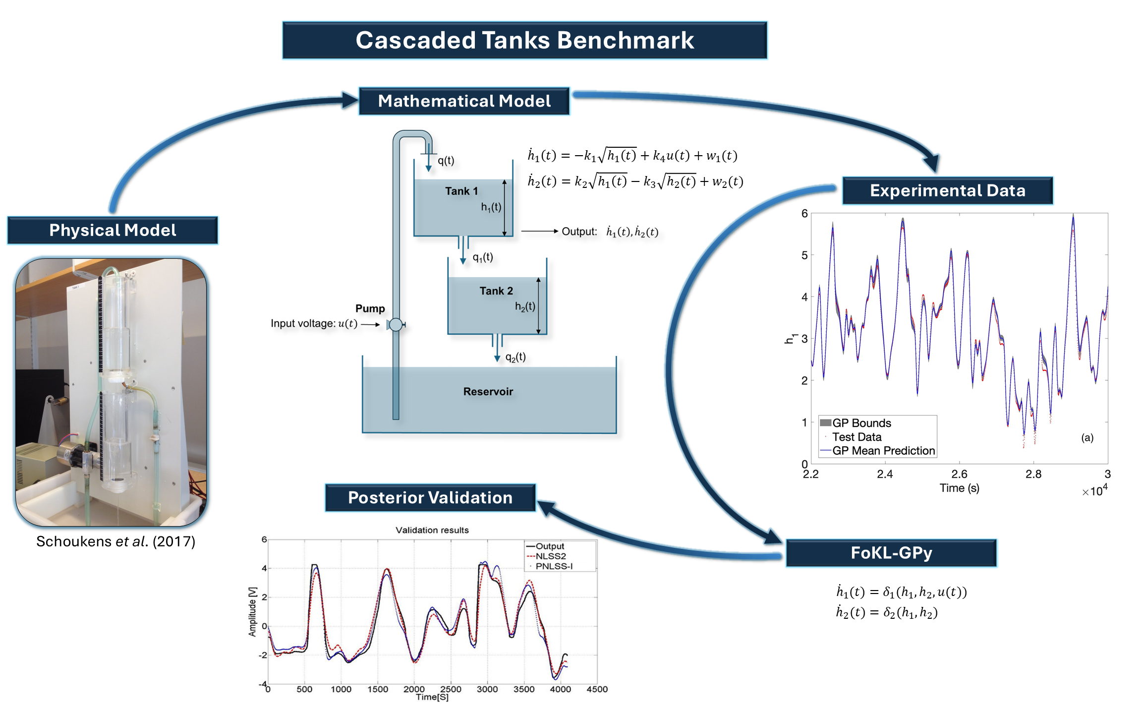
Cascaded Tanks Benchmark: An Embedded Modeling Approach
The cascaded tanks system is a fluid level control system consisting of two cascaded tanks with free outlets, the upper
tank (tank 1) is fed by a pump. The input signal controls the water pump that pumps the water from a reservoir into the upper
water tank. The water of the upper water tank flows through a small opening into the lower water tank (tank 2), and finally
through a small opening from the lower water tank back into the reservoir.
This figure illustrates the hybrid modeling process using the cascaded tanks benchmark, a standard testbed in system
identification and control.
Physical Model
The experimental setup consists of two vertically stacked water tanks with a controlled input flow, demonstrating a simple
yet dynamic physical process. The water levels in the tanks are influenced by the pump voltage input and gravity-driven flow
between tanks.
Mathematical Model
The process is governed by nonlinear ordinary differential equations describing the rate of change of water levels h1(t) and
h2(t). These equations reflect both the physical principles (e.g., outflow proportional to the square root of height) and
external inputs, like pump voltage u(t).
Experimental Data
To validate the model, empirical data capturing the tank levels over time is collected. The graph on the right compares the
measured output with the predictions made by the model, showing the accuracy of fit.
FoKL-GPy Integration
FoKL-GPy (Forward variable selection using Karhunen-Loève decomposed Gaussian Processes in Python) is applied to
model the residual errors between the physical model and experimental observations. Instead of discarding model
mismatches as noise, FoKL-GPy learns the residuals δ_1 and δ_2 as functions of system states and inputs. This enables
enhanced modeling of unknown or complex dynamics not captured by the first-principles model.
Posterior Validation
The resulting embedded model, yields more accurate predictions with quantified
uncertainties.
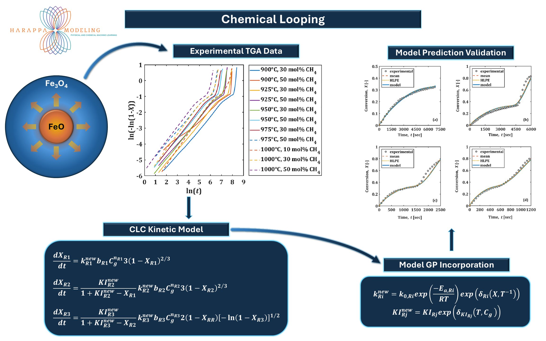
Reduction of Fe-Based Oxygen Carriers for Chemical Looping Combustion
This example presents a hybrid modeling framework to describe and predict the reduction kinetics of iron oxide-based
oxygen carriers during chemical looping with methane. The graphic illustrates the reduction of Fe_3O_4 to FeO using methane
(CH_4), a common step in chemical looping combustion (CLC).
Experimental Data
Experimental TGA data shows methane concentration and temperature effects on conversion (plotted as ln(ln(1/(1–X))) vs
ln(t)), suggesting a shrinking core or similar kinetic model.
Kinetic Modeling
Equations define the rate of conversion for different steps/phases (XR1, XR2, XR3), considering gas concentration, reaction
orders, and effective surface areas. A detailed kinetic model is constructed to describe the evolution of conversion with
each stage governed by its own rate constant and kinetic parameters.
Model Enhancement
Gaussian Process (GP) models are embedded within the kinetic expressions to account for complex, potentially
unmodeled dependencies on temperature, conversion, and gas composition. These data-driven corrections augment the
Arrhenius-based rate constants and equilibrium terms, allowing for improved parameter generalization over broader
operating conditions.
Model Validation
Comparisons between experimental and predicted conversion profiles across several scenarios confirm the model's
accuracy. The GP-enhanced kinetic model not only improves predictive accuracy but also enables robust extrapolation to
unseen conditions, including the correct prediction of the location and sharpness of the sudden change in kinetics that occurs when the reaction front reaches the surface of the particle.
the paper